This is a small project where I mess around with procedural generation and the creation of various 3D meshes for random mazes. As the end goal of the project was the creation of clean meshes, the first challenge I faced was having to consider a reasonable abstraction for the idea of a maze. There are multiple ways I can go about representing the positions of the walls and each one comes with a few advantages and disadvantages. The two options I considered most seriously, were either treating the maze as a graph and storing it as an adjacency array or treating it like a binary matrix where 1’s represent walls and 0’s represent clear passages. In my first implementation, I chose the latter, so I’ll go over its relative pros and cons first.
The primary advantage of this comes from the simplicity of visualising the maze and also converting it a mesh. As the positions of all the walls is explicit, you can construct the mesh simply by iterating over each cell in the matrix and placing a voxel everywhere there is a 1.
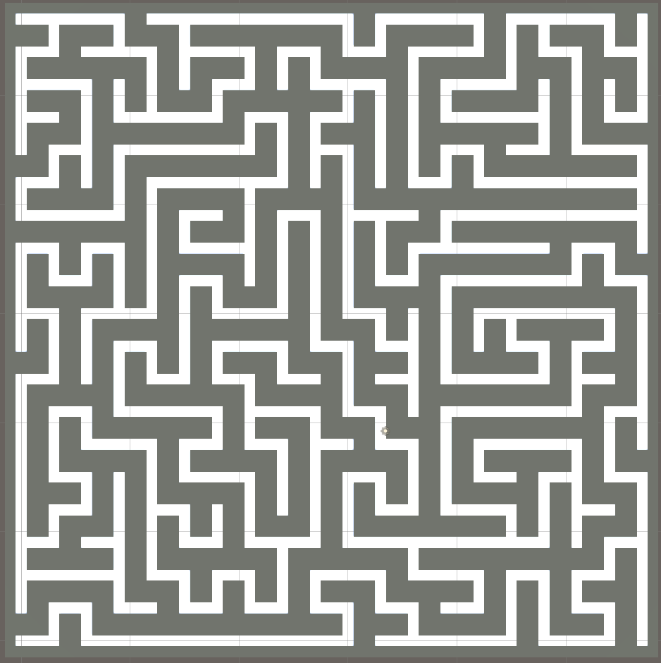
The first problem, which is immediately obvious from the image, is that the walls will feel unnaturally thick. In addition to this, is the problem of how this abstraction will work when expanding into higher dimensions. For example, when trying to construct a maze on the surface of a cube, the connections in the maze become awkward very fast. The logical way of doing this is to treat it as six 2D mazes, which each represent a single face of the cube. Then you have to manually write a mapping which allows each of these faces to link together making sure the direction and orientation of each shared edges between faces is aligned correctly. While this is possible to do, it very much limits the types of surfaces which can be modelled without doing a painstakingly tedious mapping between various 2D arrays. The final reason I chose to switch representations, was that this way of storing the state of the maze makes it awkward to implement graph-based algorithms, to do things such as solving the maze or analysing it in a more mathematical way.
The graph-based adjacency array representation makes up for the all the shortcomings of the binary matrix model, this however, does not by any means, mean that this is a perfect representation. The biggest challenge of this model comes from the fact that the existence of the walls is implicit, which means that you can only tell if a wall exists between two adjacent cells by checking to see if there is an edge between them. On top of this comes from the fact that for logical consistency this must be an undirected graph otherwise you would get disagreement on whether there is a wall between two cells or not. In addition, when constructing the maze by iterating over each cell, there is nothing within the representation which implies which cell has ownership of a wall meaning a naïve implementation will lead to duplicate walls being created causing z-fighting and other awkward artifacts.
Now that a representation is established, the next thing I needed to do was to scramble the maze. The way I did this was by starting each cell as being unconnected and then running a recursive DFS where a random neighbour is picked to have the wall removed between them and then proceeding from that cell. This method requires you to keep track of every cell you have visited to ensure that you don’t remove all the walls on a cell.
def randomise(self, self):
    visited = set()

    def dfs(cell):
        visited.add(cell)
        neighbours = list(self.neighbours(cell))
        rand.shuffle(neighbours)

        for neighbour in neighbours:
            if neighbour not in visited:
                self.connect(cell, neighbour)
                dfs(neighbour)

    dfs(start)
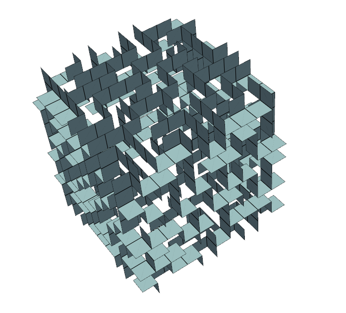
With the abstract maze finished, I can finally move onto the part of the project I found most interesting which is the generation of the mesh for different surfaces. The first type is a cubic maze, which can either be as represented as an interconnected set of 2D mazes covering the surface, or as a fully 3D maze with 6 movement options at each point in the maze. With the graphical model of the maze, I can consider these to be almost identical as I can generate the surface model using the exact same logic as the 3D maze but with the exception that I only add a cell to the graph if it lies on the surface of the cube.
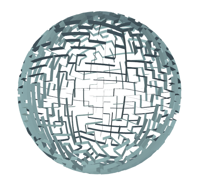
The other version, which I personally find more visually and mathematically interesting, is the spherical maze. For this to work, I need to need to find a semi regular quadrilateral tiling for a sphere. A neat solution I found for this was a projection which maps evenly distributed points on the surface of a cube onto the surface of a sphere while minimising the inevitable warping caused by such an operation. If you would like to utilise this projection I would recommend reading this blog post.
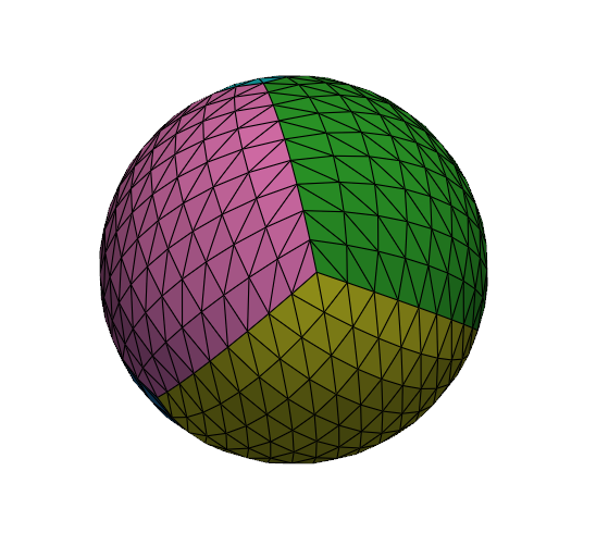
As you can see this subdivides the sphere into a series of quadrilateral cells whose adjacencies perfectly align with the cubic representation. This means that I can map the exact type of maze I used earlier directly onto the sphere with no adjustments to its abstract representation! Generating the mesh for this is a little more complex than for the cube, as the vertices which make up the walls are no longer just at fixed distance from a particular face. To align the top vertices of the wall I instead have to take the direction vector of the base of the wall relative to the sphere and scale it in that direction. However, with this done I can now arbitrarily generate spherical mazes which I hope to incorporate into a game someday.